Papero

Wednesday, 6 August 2025 at 9:13 am

---

Papero is a generative art project. It started in js in 2021 and has since had many incarnations.

The current incarnation can be found here.

This blog post is going to cover some implementations and results from over the years, as well as discussing some of the algorithms that generate the images.

I have made an interactive demo of this project, where you can generate new images with these algorithms, which you can find here.

Spiral

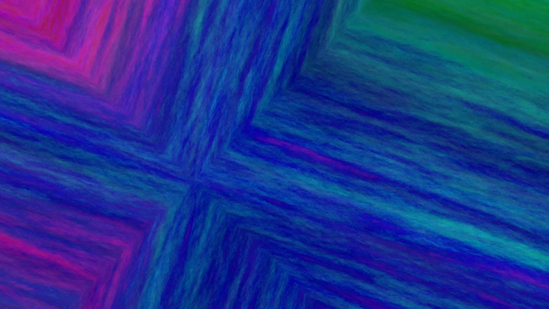
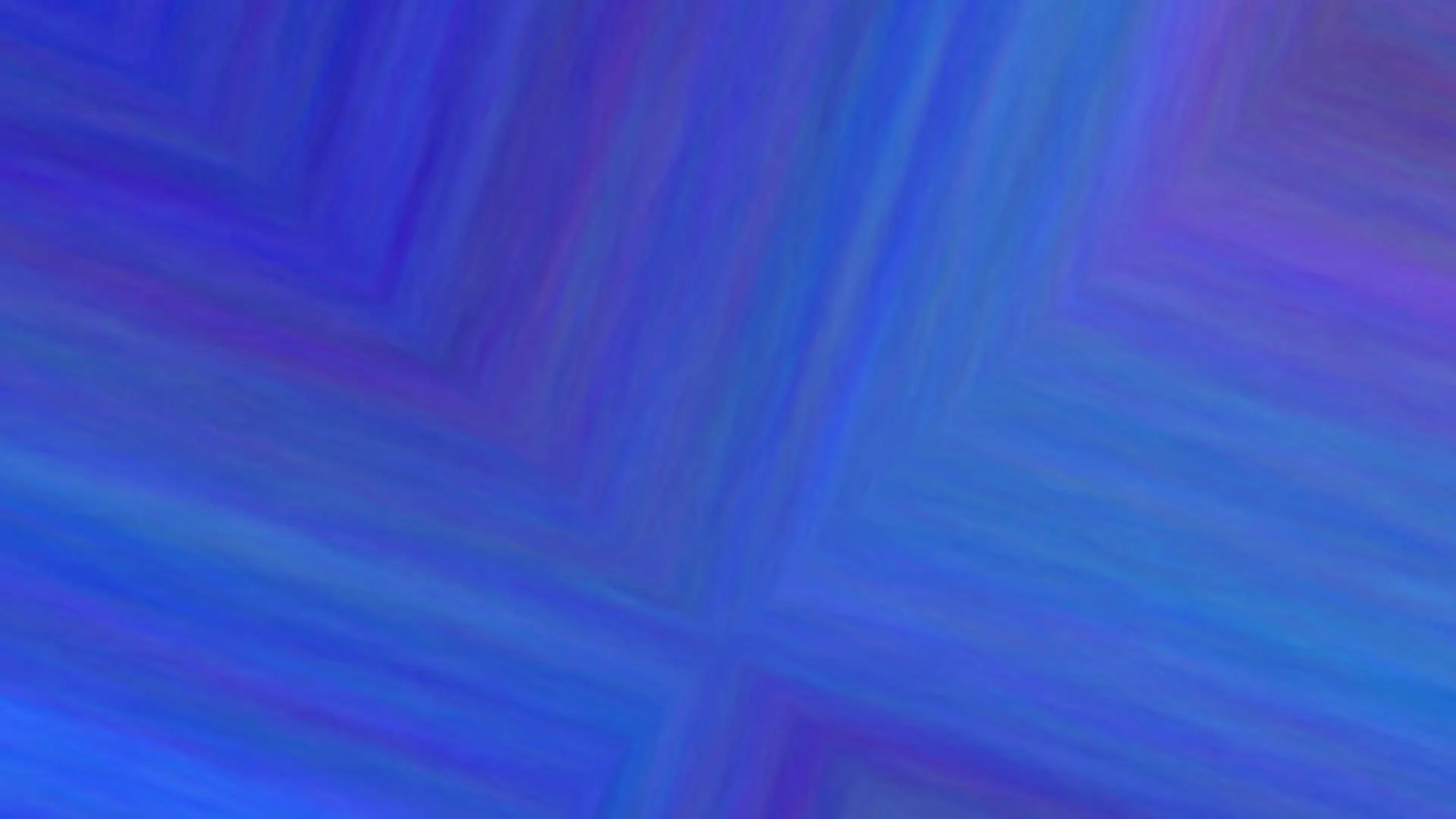
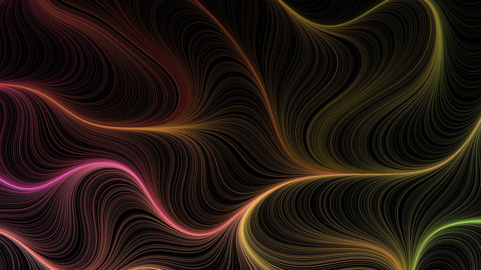
The original papero algorithm was conceived in 2021 and is now called spiral. Spiral works by walking through the image in a spiral, setting each pixel to the average of the filled pixels around it. The image starts off with one pixel, and then the walk begins going clockwise around the starting pixel repeating until the entire image is filled in. This algorithm sounds boring, and it is, in this state the entire image would end up the same colour as the starting pixel. However, if you just change the colour of the new pixel to be the average of the filled pixels around it, plus some slight randomness, the image becomes a chaotic and beautiful swirl of colour.

The oldest render from spiral I can find is from April 2023. Here it is:

The pseudocode for that algorithm looks like this:

fn generate() -> Image {
    let mut image = Image::new();

    let (mut x, mut y) = random_pixel_near_middle();

    let initial_colour = random_colour();

    image.put_pixel(x, y, initial_colour);

    // This code moves 1, then 3, then 5, etc
    // This facilitates a spiral that never hits itself.
    for move_length in 1..(max(width, height) * 2).step_by(2) {
        for _right in 0..move_length {
            spiral_iteration(&mut image, (&mut x, &mut y), Direction::Right);
        }
        for _down in 0..move_length {
            spiral_iteration(&mut image, (&mut x, &mut y), Direction::Down);
        }
        for _left in 0..(move_length + 1) {
            spiral_iteration(&mut image, (&mut x, &mut y), Direction::Left);
        }
        for _up in 0..(move_length + 1) {
            spiral_iteration(&mut image, (&mut x, &mut y), Direction::Up);
        }
    }

    return image;
}

fn spiral_iteration(image: &mut Image, (x,y): (&mut u32, &mut u32), dir: Direction) {
    (x, y) = (x, y) + dir.move_in_direction();
    if !image.in_bounds(*x, *y) {
        return;
    }
    let colour = avg_adjacent_filled(image, *x, *y);
    image.set_pixel(*x, *y, colour);
}

Here is a render of an implementation of the same algorithm from 2025.

Fractals

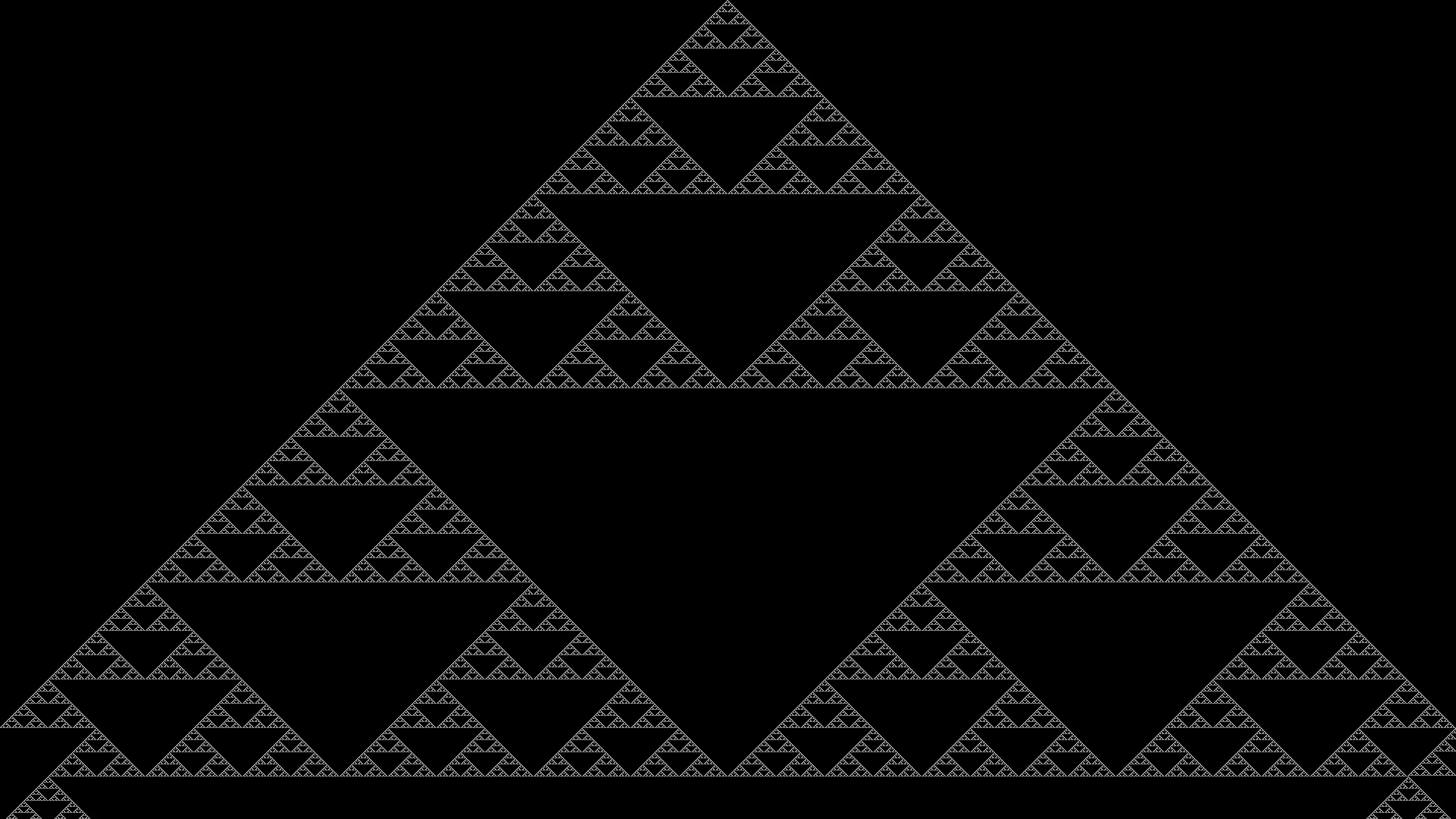
One of the next interesting experiments was with fractals. I was originally very interested in Sierpinski’s Triangle, originally coding it in python with Turtle. The performance of that algorithm was terrible, so I switched to doing it with pixels and doing the computation via Pascal’s triangle, since Pascal’s triangle mod 2 is the same as Sierpinski’s triangle. I have an interactive project that explores what it look like when you change this base here.

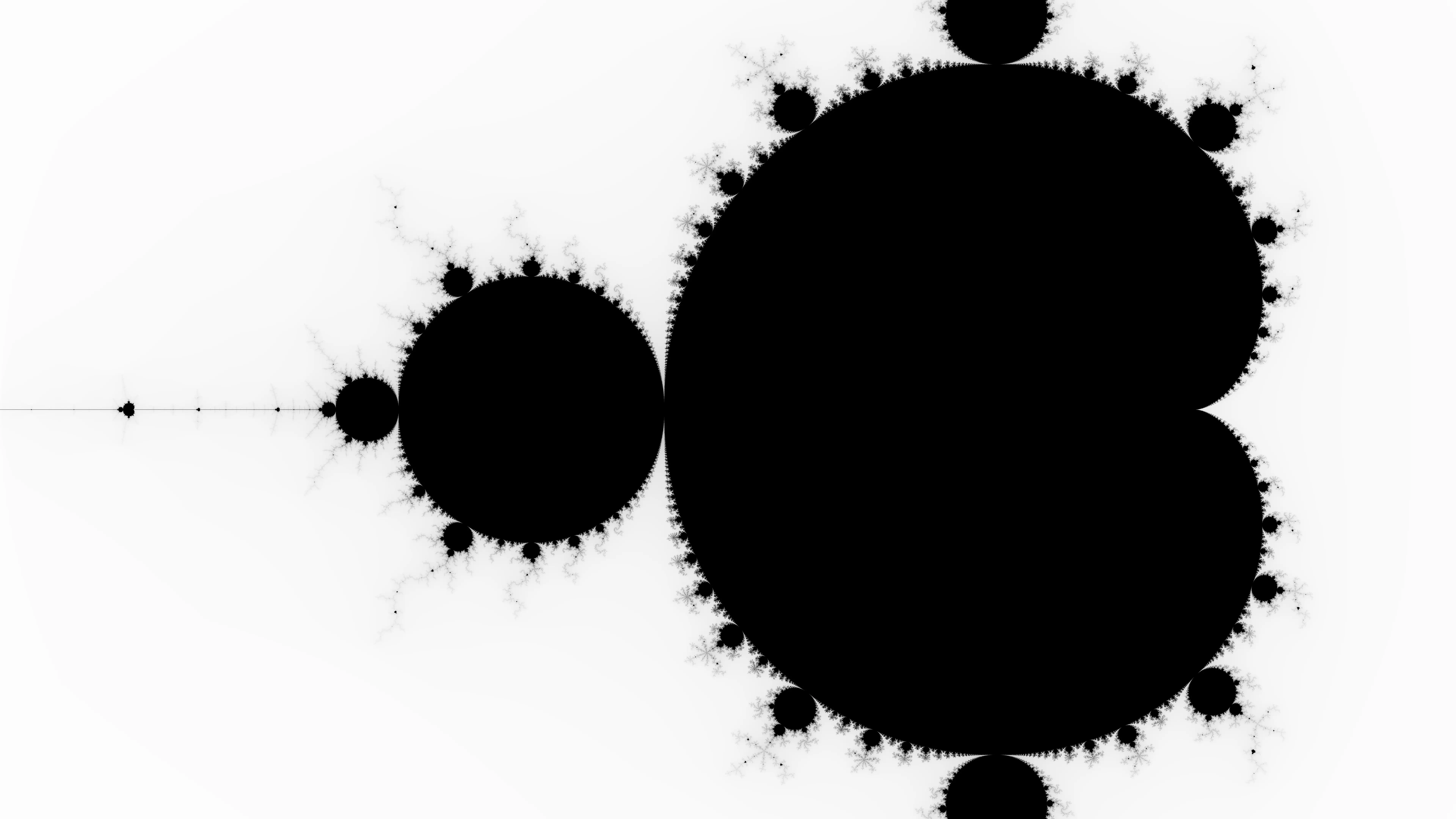
Another famous fractal is the Mandelbrot set. I have spent hours tuning the functions that choose the colour for these visualisations.

To calculate the mandelbrot set, you the pixel co-ordinates (x, y) to the complex number $c = x + yi$ (plus some shifting and scaling so that you can see the desired range).

You then iterate $z_n = z_{n-1}^2 + c$ with $z_0 = 0$.

Here is the full mandelbrot set in black and white:

Here it is in a closeup:

Here is the “inverted mandelbrot set” which can be found by mapping $c \rightarrow \frac{1}{c}$. Credit to Paul Bourke for the idea.

The Juila set, which is a variation on the Mandelbrot set, wherein $c$ is some fixed number, and $z_0 = x + yi$.

Below is the Julia set with $c=0.355 + 0.355i$:

Bitwise Images

I then had another fascination with images that were produced through simple bitwise and mathematical operations on their co-ordinates.

If you consider that a colour is simply three consecutive bytes, then you can work with colours as if they were an unsigned 24 bit integer, performing bitwise and mathematical operations exactly as you would expect. Often this results in only the lower bits being calculated since the normal width of an image ~2K pixels is much less than the number of colours ($2^{24} \approx 16.8M$). Therefore in these images I typically scaled the co-ordinates so that $x, y \in [0, 2^{24})$

One of the simplest bitwise operations is AND, and by performing it on the co-ordinates of an image, you get this fascinating image:

Here’s another made with the same process by with OR:

And another made by squaring x and y and then XOR-ing them together, it’s probably my favourite of the three:

// x, y are already scaled to the range [0, 2^24)
fn sq_xor(x:u32, y:u32) -> Color {
    let c = x.pow(2).bitxor(y.pow(2));
    u32_to_colour(c as u32)
}

As for the mathematical operations, I considered the formula for a circle $x^2 + x^2 = r^2$, and figured it would be interesting to try. Thus the $x^2 + y^2$ image was born.

Here it is with (0, 0) in the top left, this is normal for images.

Here it is with (0, 0) in the centre, this is not normal for images but makes it look nicer.

For both of these images I recommend you open them in a new tab so you can properly zoom in and pan around. They have a lot of strange details and screen door effect.

These final images were generated by an algorithm that has been lost to time. All I know is that the bands of colour were due to intentional rounding halfway through the calculation, and it has something to do with a cuberoot.

Here it is with (0, 0) in the top left:

And here with (0, 0) in the center:

How cool!

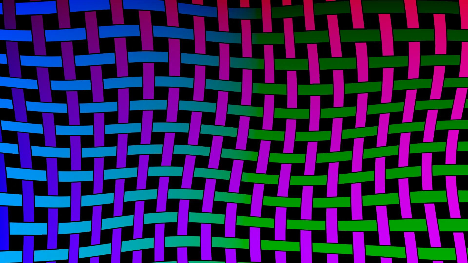
You can find lots more algorithms at the GitHub here.

Here is just a taste:

Thanks for reading.

Gabriel